how to draw protein 3d structure

When working with poly peptide 3D structures, a contact map is usually divers as a binary matrix with the rows and columns representing the residues of two dissimilar bondage. Each matrix element is one/True if the blastoff carbon distance between the associated residues is less than some threshold (such as half dozen angstroms), or null/Faux if the residues are far away.

This means that the showtime step in computing a contact map betwixt to protein chains, is to calculate the alpha carbon altitude between pair of their residues. BioPython's Bio.PDB module includes lawmaking to load PDB files and calculate these distances.

An example PDB file

I have choosen to look at PDB file 1XI4, which is the clathrin muzzle lattice (described in more detail as the PDB's April 2007 Molecule of the Month). If you download the default PDB file (merely over 1MB) you only get part of the circuitous brawl structure made upwardly of just nine clathrin heavy bondage (Bondage A to I in the PDB file) and nine clathrin lite bondage (Bondage J to R). For drawing pretty pictures you desire to download and uncompress the Biological Unit of measurement Coordinates instead (once uncompressed this is a xiv MB file). In both cases, only the alpha carbon atoms are listed in the PDB file, and there are no annotated alpha helices or beta sheets. This means that virtually of the fancy protein visualisations available in RasMol or VMD won't work - so the illustration on the left is from the PDB website.

Calculating the distances and contact map

As with most python scripts, this one starts by importing some libraries, and setting upward some constants:

          import Bio.PDB import numpy  pdb_code = "1XI4" pdb_filename = "1XI4.pdb" #not the full cage!        

Now we define a simple role which returns the distance between two residues' alpha carbon atoms, and a 2d part which uses this to calculate an entire distance matrix:

          def calc_residue_dist(residue_one, residue_two) :     """Returns the C-alpha distance between two residues"""     diff_vector  = residue_one["CA"].coord - residue_two["CA"].coord     return numpy.sqrt(numpy.sum(diff_vector * diff_vector))  def calc_dist_matrix(chain_one, chain_two) :     """Returns a matrix of C-alpha distances between two chains"""     answer = numpy.zeros((len(chain_one), len(chain_two)), numpy.float)     for row, residue_one in enumerate(chain_one) :         for col, residue_two in enumerate(chain_two) :             answer[row, col] = calc_residue_dist(residue_one, residue_two)     return respond        

And then the PDB file is read into the variable structure using Bio.PDB.PDBParser(). This provides a list of the models in the PDB file (in this case, simply one as NMR was not used).

          structure = Bio.PDB.PDBParser().get_structure(pdb_code, pdb_filename) model = construction[0]        

Within this model there are in fact 18 chains (nine heavy and nine low-cal). The post-obit code calculates the altitude matrix between low-cal chain D and heavy chain M - called considering they are in close contact (and also positioned in the eye of the sub-unit of measurement of the total muzzle represented in the PDB file).

          dist_matrix = calc_dist_matrix(model["D"], model["Thousand"]) contact_map = dist_matrix < 12.0        

The final line turned the distance matrix (held equally a float array) into contact map (equally a logical array) using a threshold of 12 angstroms.

Now, 1 obvious question is what is the range of distances in our matrix? You tin can try using the python built in min() and max() functions merely the don't requite the expected behaviour for Numeric arrays. Instead, we must employ numpy'due south own functions:

          impress "Minimum distance", numpy.min(dist_matrix) impress "Maximum distance", numpy.max(dist_matrix)                  

This gives the following output:

          Minimum distance four.62857341766 Maximum distance 201.617782593        

The closest residues plow out to be residue Asn155 in low-cal concatenation D, and Leu1504 in heavy chain M. In fact in that location are but a couple of pairs closer than 6 angstroms - simply its not very easy to come across this from a massive matrix like this.

Drawing the altitude matrix in Python

I'll show another method in a moment, just first lets use the python library Matplotlib to exercise some plotting:

          import pylab pylab.matshow(numpy.transpose(dist_matrix)) pylab.colorbar() pylab.show()        

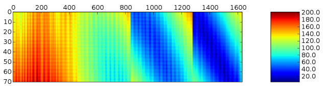
As you can see, the light chain (vertical axis) is in contact with only the C-terminal region of the heavy concatenation (horizontal axis). You can too see some banding in the distance plot, which yous tin probably explain in terms of the secondary structure.

You might want to look at pylab.pcolor() instead of pylab.matshow(), for one thing the y-axis runs the other way up.

At present lets testify the contact map (which is a boolean matrix, and then with merely two values a colour central is a bit redundant), and while we're at information technology, lets change the color scheme:

          pylab.fall() pylab.imshow(numpy.transpose(contact_map)) pylab.evidence()        

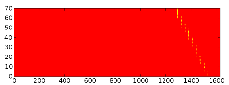
Pretty! Still, the vertical axis needs relabelling for some reason...

Cartoon a contour plot of the distances

This is really overkill on this example where plotting an array of little coloured squares is more than enough, but I went on to show the distance map every bit a contour plot. It seemed similar a logical next step - especially as I have already worked out how to do depict this sort of thing in R (e.g. Contour Plots of Matrix Data in R) and you can telephone call R from python using rpy.

This chip of code was used to turn the distance matrix into a contour plot:

This used to work fine with Numeric instead of numpy, merely perhaps my copy of rpy is out of engagement as it complains "no proper 'z' matrix specified".

          import rpy rpy.r.library("gplots") rpy.r.png("1XI4_D-1000.png", width=600, acme=300) rpy.r.filled_contour(10=rpy.r("1:1630"), \                      # residue numbers in heavy chain                      y=rpy.r("95:164"), \                      # rest numbers in light concatenation                      z=dist_matrix, \                      xlab="Heavy chain Grand", \                      ylab="Low-cal concatenation D", \                      levels=[0,6,14,20,200], \                      col=rpy.r.colorpanel(4, "red", "white"),                      principal="Protein Contact Map for Clathrin Cage") rpy.r.dev_off() # close the image file        

And here is the resulting image, observe over again the all of the light concatenation is in contact with the C-terminal region of the heavy chain - maybe information technology would be more interesting to produce a plot of simply that region... The colour primal changes at 6, 14, and 20 angstroms:

bryantsonew1991.blogspot.com

Source: https://warwick.ac.uk/fac/sci/moac/people/students/peter_cock/python/protein_contact_map/

Share this post